LESSON 4: POINT PATTERN ANALYSIS

Lesson 4 Overview

Introduction

In the previous lesson we saw how a spatial process can be described in mathematical terms so that the patterns it is expected to produce can be predicted. In this lesson we apply this knowledge to the analysis of point patterns. Point pattern analysis is the application in which these ideas are most thoroughly developed, so it is the best place to learn about this approach.

Point pattern analysis has become an extremely important application in recent years, particularly in crime analysis, in epidemiology, and in facility location planning and management. Point pattern analysis also goes all the way back to the very beginning of spatial analysis in Dr. John Snow's work on the London cholera epidemic of 1854.

Learning Objectives

By the end of this lesson, you should be able to

1. define point pattern analysis and list the conditions necessary for it to work well
2. explain how quadrat analysis of a point pattern is performed and distinguish between quadrat census and a quadrat sampling methods
3. discuss relevant factors in determining an appropriate quadrat size for point pattern analysis
4. describe in outline kernel density estimation and understand how it transforms point data into a field representation
5. describe distance-based measures of point patterns (mean nearest neighbor distance and the G, F and K functions)
6. explain how distance-based methods of point pattern measurement are derived from a distance matrix
7. describe how the independent random process and expected values of point pattern measures are used to evaluate point patterns, and to make statistical statements about point patterns
8. explain how Monte Carlo methods are used when analytical results for spatial processes are difficult to derive
9. justify the stochastic process approach to spatial statistical analysis
10. discuss the merits of point pattern analysis versus cluster detection, and outline the issues involved in real world applications of these methods

Reading Assignment

This week the reading is detailed, demanding, and long. I therefore recommend that you start it as soon as possible, and also that you read the material twice. First time through, you should quickly skim the material to become familiar with the overall plan. On the second pass, you should read more closely taking note of the details. Whatever you do, don't leave the reading to the last minute this week!

• Chapter 4, "Point Pattern Analysis," pages 77-114
• Chapter 5, Section 5.1, "Practical Point Pattern Analysis," pages 115-123
  You need only read the first section of Chapter 5 (noted below), although I hope that you will find all of it useful as a guide to current and future developments in point pattern analysis.

After you've completed the reading, or at the very least skimmed the material, get back online and supplement your reading from the commentary material, then test your knowledge with the self-test quizzes.

Lesson 4 Deliverables

This lesson is one week in length. The following items must be completed by the end of the week. See the Calendar tab, above, for the specific date.

1. Complete the two self-test quizzes satisfactorily (you have an unlimited number of attempts and must score 90% or more).
2. Complete the Project 4 activities. This involves running and interpretting point pattern analysis of some crime data for St Louis. (The materials for Project 4 can be found under the Lessons tab, in the Lesson 4 folder.)
3. There is no specific activity in the quarter-long project this week, as the core of this week's lesson will keep you busy enough. However, don't forget that you have to submit a review of two other research proposals next week—I will tell you which ones this week.

Questions?

If you have any questions now or at any point during this lesson, please feel free to post them to the Lesson 4 thread on the Lesson Content Discussion Forum .(That Discussion Forum can be accessed at any time by clicking on the Communicate tab, above, and then scrolling down to the Discussion Forums section.)

LESSON 4: POINT PATTERN ANALYSIS

Commentary - Chapter 4, "Point Pattern Analysis"

Section 4.2, "Describing a point pattern," pages 79-81

It should be pointed out that the distinction between first- and second-order effects is a fine one. In fact, it is often scale-dependent, and often an analytical convenience, rather than a hard and fast distinction. This becomes particularly clear when you realize that an effect that is first-order at one scale may become second-order at a smaller scale (that is, when you 'zoom out').

The simplest example of this is when a (say) east-west steady rise in land elevation viewed at a regional scale is first-order, but zooming out to the continental scale, this trend becomes a more localized topographic feature. This is yet another example of the scale-dependence effects inherent in spatial analysis and noted in Lesson 1.

Section 4.3, "Density-based point pattern measures," pages 81-88

It is worth emphasizing the point that quadrats need not be square, although it is rare for them not to be.

With regard to kernel density estimation (KDE) it is worth pointing out the strongly scale-dependent nature of this analysis method. This becomes apparent when we view the effect of varying the KDE bandwidth on the estimated event density map in the following sequence of maps, all generated from the same pattern of homicide events in St. Louis, Missouri downtown in 1982.

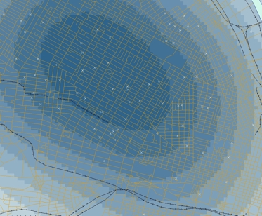
Using a large KDE bandwidth results in a very generalized impression of the event density.

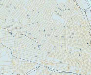
The map generated using a small KDE bandwidth is also problematic, as it focuses too much on individual events.

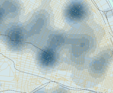
An intermediate choice of bandwidth results in a more satisfactory map that enables distinct regions of high density of events (clusters) to be identified.

Section 4.4, "Distance-based point pattern measures," pages 88-95

It may be helpful to briefly distinguish the four major distance methods discussed here:

1. Mean nearest neighbor distance is exactly what the name says!
2. G function is the cumulative frequency distribution of the nearest neighbor distance. It gives the probability for a specified distance, that the nearest neighbor distance to another event in the pattern will be less than the specified distance.
3. F function is the cumulative frequency distribution of the distance to the nearest event in the pattern from random locations not in the pattern.
4. K function is based on all inter-event distances, not simply nearest neighbor distances. Interpretation of the K function is tricky for the raw figures and makes more sense when statistical analysis is carried out as discussed in a later section.

It is useful to see these measures as forming a progression from least to most informative (with an accompanying rise in complexity).

Section 4.5, "Assessing point patterns statistically," pages 95-108

The measures discussed in the preceding two sections can all be tested statistically for deviations from the expected values associated with a random point process. In fact deviations from any well defined process can be tested, although the mathematics required becomes more complex.

This section simply outlines how each of the measures described in previous sections may be tested statistically. The most complex of these is the K function, where the additional concept on an L function is introduced to make it easier to detect large deviations from a random pattern.

More important, in practical terms is the Monte Carlo procedure discussed on pages 104-108. Monte Carlo methods are common in statistics generally, but are particularly useful in spatial analysis when mathematical derivation of the expected values of a pattern measure can be very difficult. Instead of trying to derive analytical results, we simply resort to the computer's ability to randomly generate many patterns according to the process description we have in mind, and then compare our observed result to the simulated distribution of results. This approach is explored in more detail in the project for this lesson.

LESSON 4: POINT PATTERN ANALYSIS

Commentary - Chapter 5, Section 5.1, "Point Pattern Analysis Versus Cluster Detection"

The key issue here is that classic point pattern analysis allows us to say that a pattern is ' evenly-spaced' or ' clustered' relative to some null spatial process (usually the independent random process), but it does not allow us to say where the pattern is clustered. This is important in most real world applications. A criminal investigator takes it for granted that crime is more common at particular 'hotspots', i.e., that the pattern is clustered, so statistical confirmation of this assumption might be nice, but it is not particularly useful. However, an indication of where the crime hotspots are located is definitely useful.

The problem is that detecting clusters in the presence of background variation in the affected population is very difficult. This is especially so for rare events. You can get some idea of the degree of difficulty from the description of the Geographical Analysis Machine (GAM) on pages 119-122. Although GAM has not been widely adopted by epidemiologists, the approach suggested by it was ground-breaking and other more recent tools use very similar methods. (See the optional 'Try This' box below for more on this.)

The basic idea is very simple: repeatedly examine circular areas on the map and compare the observed number of events of interest to the number that would be expected under some null hypothesis (usually spatial randomness). Tag all those circles that are statistically unusual. That's it!

Three things make this conceptually simple procedure tricky.

• First, is the statistical theory associated with determining an expected number of eventsperhaps dependent on a number of spatially varying covariates of the events of interest, such as populations in different age subgroups. Thus, for a disease (say) associated with older members of the population, we would naturally expect to see more cases of the disease in places where more older people live. This has to be accounted for in determination of the number of events expected.
• Second, there are some conceptual difficulties in carrying out multiple statistical significance tests on a series of (usually) overlapping circles. The rather sloppy statistical theory in the original presentation of the GAM goes a long way to explaining the reluctance of statistical epidemiologists to adopt the tool, even though more recent tools are rather similar.
• Third, is the enormous amount of computation required for exhaustive searching for clusters. This is especially so if stringent levels of statistical significance are required, since many more Monte Carlo simulation runs are then required.

LESSON 4: POINT PATTERN ANALYSIS

Final Activities for Lesson 4

Now that you've completed the readings and self-test quizzes for this lesson, it is time to apply what you've learned!

The following links will open in a new browser window.

1. Complete Project 4, in which we will analyze crime data for St Louis, in order to demonstrate some of the point pattern analysis methods that have been discussed in this week's lesson. (When you are done reviewing this Web page, click on the "Next" link, above, to begin Project 4. The materials for Project 4 can also be found under the Lessons tab, in the Lesson 4 folder.)
2. Continue the Quarter-long Project by reviewing the Week 4 directions. ( This link opens in a new window - The materials for the Quarter-long Project can be also be found under the Lessons tab.)

PROJECT 4: POINT PATTERN ANALYSIS

Overview

Background

In this week's project you will use some of the point pattern analysis tools available in ArcGIS together with one we've made specially for this course to investigate a point pattern of crime events in St. Louis.

Project Resources

The ArcMap template file and data files you need for Project 4 are available here for download. If you have any difficulty downloading these files, please contact me.

• PtPatternAnalysis_v9.2.mxt is an ArcMap template file with additional custom functionality to support quadrat analysis. (That file is 783 Kb and will take approximately 2 minutes to download over a 56 Kbps modem.) Many, many thanks to Jim Detwiler for programming this file!
• project4_ptData.zip is a zip file that contains two shape files: gunHomicide.shp records the locations of homicides in St. Louis, Missouri, in 1982; and attemptedStreetRobbery.shp, which records the location of incidents of attempted 'non-residential burglary' over the same period. (That file is 14 Kb and should be quick to download even over a 56 Kbps modem. Once you have downloaded the file, double-click on the project4_ptData.zip file to launch WinZip, PKZip, 7-Zip, or another file compression utility. Follow your software's prompts to decompress the file.)
• project4_data.zip is a zipped version of an ArcGIS geodatabase file StLouisCrime.mdb , with layers of background topography, principally the street network, for St. Louis, Missouri. This serves no actual purpose in the analysis as such, but gives some context for the exercise, and may help in your discussions of results. (That file is 1.9 Mb and will take around 5 minutes to download over a 56 Kbps modem. Once you have downloaded the file, double-click on the project4_data.zip file to launch WinZip, PKZip, 7-Zip, or another file compression utility. Follow your software's prompts to decompress the file.)

Open a new ArcMap map from the .mxt template file. Do this either:

• By double-clicking on PtPatternAnalysis_v9.mxt in the explorer, or
• From ArcMap by selecting File - New... and navigating to the PtPatternAnalysis.mxt template, or
• From the ArcMap start up dialog, by selecting the Start Using ArcMap with a Template option.

You should immediately set the File - Map Properties... - Data Source Options... to Store Relative Path Names, and save the new project (even with no data) to a new .mxd file.

Once you've done that, load in the shape files from project4_Ptdata.zip along with the background layers in the StLouisCrime.mdb file. .

Summary of Project 4 Deliverables

For Project 4, the items you are required to submit are as follows:

• Create and insert a map showing standard deviational ellipses for the two crime patterns and commentary on the relative locations of the two patterns.
• Calculate nearest neighbor distance statistics for both crime patterns and comment on these results.
• Create and insert maps of quadrat analyses of the two crime patterns, along with commentary on each, and details of the analysis results in each case. You have to choose the quadrat size and analysis method (census- or sample-based) and should provide some explanation of your choices.
• Create density maps of the gunHomicide and attemptedStreetRobbery data. Insert the maps into your write-up along with commentary explaining your choice of parameters, particularly the bandwidth.
• Finally, comment on the study area in all these examples: it has effectively been set for you by the dataset. Do you think more extensive data would lead to different conclusions? How would the results be affected?

Questions?

If you have any questions now or at any point during this project, please feel free to post them to the Project 4 thread on the Project Discussion Forum. (That Discussion Forum can be accessed at any time by clicking on the In Touch tab, above, and then scrolling down to the Discussion Forums section.)

Ready to continue? Click on the "Next" link, above, to continue with this project.

PROJECT 4: POINT PATTERN ANALYSIS

Standard Deviation Ellipses for the Crime Patterns

Before conducting any analysis it is sensible to get an overall feel for the two crime patterns. The ArcGIS Toolbox provides some simple tools for this including standard deviation ellipses. To open the toolbox, click on the button in the main application toolbar. In the hierarchical list of toolboxes that appears, you will find the standard deviation ellipse tool in the Spatial Statistics Tools - Measuring Geographic Distributions toolbox. Operation of the tool is self-explanatory, so I'll leave it to you to figure things out.

Create a map showing standard deviational ellipses for the two crime patterns and commentary on the relative locations of the two patterns.

Ready to continue? Click on the "Next" link, above, to continue with this project.

PROJECT 4: POINT PATTERN ANALYSIS

Mean Nearest Neighbor Distance Analysis for the Crime Patterns

Next conduct mean nearest neighbor distance analysis of the crime patterns. You will find the required tool in the Spatial Statistics Toolbox in the 'Analyzing Patterns' subset. Operation of this tool is self-explanatory, so I'll allow you to figure it out for yourself.

Calculate nearest neighbor distance statistics for both crime patterns and report and comment on the results.

Ready to continue? Click on the "Next" link, above, to continue with this project.

PROJECT 4: POINT PATTERN ANALYSIS

Familiarization with the Quadrat Analysis Tool

As part of this project, a quadrat analysis tool has been developed by Jim Detwiler. This page explains its operation.

The quadrat analysis tool is available in any map file created from the PtPatternAnalysis_v9.mxt template and appears as a toolbar:

The Point Pattern Analysis toolbar

If the toolbar is not available, right-click on the ArcMap program window and select it from the drop-down menu:

The right-click menu that allows you to enable Point Pattern Analysis

Defining the study area

1. To define a study area for analysis click on the New Rectangle button then mouse-drag a rectangle across from one corner to the diagonally opposite corner of the rectangular study area you wish to define. This creates a graphic object that is currently selected.
2. To define this as the study area for either census or grid-based quadrat analysis click on Census - Create Grid or on Sampling - Define Study Area. What happens next is explained in the next two sections.

If you want to define a quadrat analysis with precise dimensions, then before clicking on the Create Grid or Define Study Area menu items, you should right-click on the rectangle, and select Properties - Size and Position and define the width and height you want. You can also define how the rectangle is drawn. Making it transparent will make it easier to position it precisely where you want by dragging.

Defining a grid for census-based analysis and running the analysis

The Census - Create Grid option asks you to define the parameters for a regular rectangular grid inside the study area rectangle just defined. This is done in terms of the required numbers of rows and columns of (rectangular) quadrats.

Once you have defined the number of rows and columns, a new shapefile will be created and added to the map.

1. To use the new shapefile for quadrat analysis, click Census - Run Analysis. In the dialog that appears specify the point layer containing the pattern to analyze, specify whether or not to use an attribute of each point as an event count, and specify the shapefile containing the census quadrats to use. Then click on Calculate Stats to run the analysis.

   

   Use this dialog to define parameters for the quadrat analysis.

2. When the analysis is complete, the following results window will appear:

   

   Results from quadrat analysis. These are formatted in a similar way to Table 4.3 on page 99 of the course text.

3. You can save the results to a text file in a spreadsheet readable format by clicking the Export button.

The analysis adds a field to the census grid shapefile named 'K' which, for each quadrat records how many events occurred in that quadrat. You may find it helpful in understanding the method to color the layer using this attribute.

Defining a quadrat for sample-based analysis

1. For sample-based analysis, once you have defined a study region with the New Rectangle tool, by clicking on Sampling - Define Study Area, you should again click on New Rectangle and draw a new rectangle, then click on Sampling - Define Quadrat to specify that this is the quadrat shape required.
2. Once both shapes are defined, click on Sampling - Run Analysis to calculate the results as for a census-based analysis.
3. When you have completed sample-based analysis, you can remove all the graphic objects it creates using the Remove Count Labels and Remove Quadrats buttons. Note that the Remove Quadrats button will leave both the study area rectangle and one quadrat intact, in case you want to repeat the analysis. You should select and delete these by hand if you want a 'clean' display.

   You can make non-rectangular quadrats for sample-based analysis using the ArcMap drawing tools. However, the Remove Quadrats button will not work properly on them, and you will have to clean up by hand.

Exporting the results to a text file and determining a p value

1. Click on Export in the Quadrat Count Statistics dialog to create a tab-separated text file summarizing the analysis results.
2. Read the tab-separated text file with a spreadsheet program to determine the p value associated with the analysis. In Openoffice.org Calc or Microsoft Excel the function required to calculate this is CHIDIST.

   You can also use a spreadsheet program to plot a histogram of the analysis results, which you may also find helpful.

Ready to continue? Click on the "Next" link, above, to continue with this project.

PROJECT 4: POINT PATTERN ANALYSIS

Quadrat Analysis of the Two Crime Patterns

Perform quadrat analyses on each of the two crime patterns. You should base your choices of study area, quadrat size and numbers of quadrats as well as the method (census- or sample-based) on the previous descriptive analyses and also on your reading of this week's lesson and its support materials. Note that it is not necessary to define a study region that includes all the events in each case. You may wish to consider the advantages (or not) of defining the same study area for each pattern.

Create maps of quadrat analyses of the two crime patterns, along with commentary on each, and details of the analysis results in each case. You have to choose the quadrat size and analysis method (census- or sample-based) and should provide some explanation of your choices.

Ready to continue? Click on the "Next" link, above, to continue with this project.

PROJECT 4: POINT PATTERN ANALYSIS

Kernel Density Analysis

In this part of the project, you use built-in ArcMap Spatial Analyst functionality to help understand the crime data. Two maps and accompanying commentary are required. Both are made using the Spatial Analyst - Density... tool.

1. First, open the Spatial Analyst - Density... tool. You will see the following dialog box:

   The density estimation dialog box. Specify parameters for kernel density estimation here (see text).

2. Specify the following parameters:
   • Input data - the point pattern data set
   • Population field - the attribute that includes a count of the number of events occurring at one location.
   • Density type - Kernel or Simple, as discussed in the text. In this project you should select Kernel .
   • Search radius - the kernel bandwidth.
   • Area units - the units that will be used in the density estimate calculation.
   • Output cell size - the resolution of the grid across which density estimates will be made.
   • Output raster - a file name for saving the analysis result permanently.
3. Use this dialog for the analyses outlined below.
   • Create density maps of the gunHomicide and attemptedStreetRobbery data. Place the maps in your write-up along with commentary explaining your choice of parameters, particularly the bandwidth.
   • Finally, comment on the study area in all these examples: it has effectively been set for you by the dataset. Do you think more extensive data would lead to different conclusions? How would the results be affected.

Ready to continue? Click on the "Next" link, above, to continue with this project.

PROJECT 4: POINT PATTERN ANALYSIS

Checklist of Project 4 Deliverables

Here is a summary of the deliverables for Project 4, to be posted as a PDF (preferably) or MS Word document. Once posted, please provide a link to the document in the discussion forum "Posted project links" thread for this week. Note that if you don't have access to any webspace for posting, that you can simply attach the document to your post to the discussion forum. Make sure you have completed each item!

1. Create a map showing standard deviational ellipses for the two crime patterns and commentary on the relative locations of the two patterns.
2. Calculate nearest neighbor distance statistics for both crime patterns and report and comment on the results.
3. Create maps of quadrat analyses of the two crime patterns, along with commentary on each, and details of the analysis results in each case. You have to choose the quadrat size and analysis method (census- or sample-based) and should provide some explanation of your choices.
4. Create density maps of the gunHomicide and attemptedStreetRobbery data. Put the maps in your write-up along with commentary explaining your choice of parameters, particularly the bandwidth.
5. Finally, comment on the study area in all these examples: it has effectively been set for you by the dataset. Do you think more extensive data would lead to different conclusions? How would the results be affected?

That's it for Project 4!

End of Project 4 - Remember, if you have any questions, post them to the appropriate Discussion Forum.

QUARTER-LONG PROJECT

Week 4: Beginning the Peer Review Process

There is no specific deliverable for this week, however you should use this week to begin the peer review process for the preliminary proposals. Early this week I will send an email letting you know which two other student's proposals you have been assigned to review. Begin by looking at the two proposals you have been assigned to review as posted on the 'Project Initial Proposal discussion board' (you can get to this by clicking on 'Previous' above). Then, simply post your comments as a response to the assigned project proposal message. Your peer reviews are due by the end of Week 5. (Although you are welcome to post them at any point between now and then.)

You should consider the following aspects in writing comments for the authors of the proposals:

• Are the goals reasonable and achievable? It is a common mistake to aim too high and attempt to do too much. Suggest possible amendments to the proposals' aims that might make them more achievable in the time frame.
• Are the data adequate for the task proposed? Do you foresee problems in obtaining or organizing the data? Suggest how these problems could be avoided.
• Are the proposed analysis methods appropriate? Suggest alternative methods, or enhancements to the proposed methods that would also help.
• Provide any additional input that you feel is appropriate. This could include suggestions for additional outputs (e.g., maps) not specifically mentioned by the author, or suggestions as to further data sources, relevant things to read, relevant other examples to look at, and so on.

Remember... you will be receiving two reviews from other students of your own proposal, so you should include the types of useful feedback that you would like to see in those commentaries. Criticism is fine, provided that it includes constructive inputs and suggestions. If something is wrong, how can it be fixed?

Meanwhile, I will be reviewing the preliminary proposals, and providing each of you with feedback and suggestions. I will aim to complete my reviews and mail them to you this week.

Questions?

If you have any questions now or at any point during this project, please feel free to post them to the Quarter-long Project Discussion Forum. (That Discussion Forum can be accessed at any time by clicking on the In Touch tab, above, and then scrolling down to the Discussion Forums section.)

That's it for the quarter-long project this week!